Today I have no fancy project and no shiny GitHub repository to show because today I want to talk about my research. As some may read in my bio, I am doing my PhD in the field of predictive maintenance (PDM). This field is directly adjacent to machine learning and fell, like many others, into the grasp of the deep learning hype. Unfortunately, long series of sensor readings are not as interesting to look at as images or intuitively understood as natural language, so PDM is not as present in the mind of the general ML crowd. Maybe this post can shed a little light on this corner of the research world.
But, this post is not only about my research. It is about the mindset an ML practitioner has to maintain when it comes to problems outside the commonly represented fields (i.e. CV and NLP). Maybe “Be aware of your data and use case.” would be a fitting tl;dr, but I think to really get what it means I have to go a bit further in my explanation. Our road map is pretty simple. First, we take a short tour of the field of PDM and define the specific task I am researching, remaining useful lifetime (RUL) estimation. Second, we investigate the problem with this task and how to alleviate it. Last, we will see how the current literature fails to do so by naïvely copying deep learning techniques from other fields.
Predictive Maintenance, Prognostics, and Remaining Useful Lifetime Estimation
Predictive maintenance (PDM) or sometimes called condition-based maintenance (CBM) a smart kind of maintenance scheduling. Instead of waiting for a machine to fail and suffer downtime, or repairing the machine in a set time interval to avoid downtime at all costs, PDM monitors the health status of the machine to anticipate failure. This aims to minimize both downtime and costs of repair. Traditionally, there are ways to predict the machine status through physical models or expert systems, but we will focus on data-driven approaches (i.e. deep neural networks).
Most times, the data used for PDM are multivariate time series. The channels of the series constitute of sensor readings during operation (e.g. vibration or temperature) or test readings done at specific time intervals. Label information is mostly provided as one label for each series. Naturally, PDM data is imbalanced in favor of data from healthy, normally running machines. Data from failing machines is much rarer, as failures should be the exception, not the norm. Benchmark datasets often contain several subsets, where the machine is the same but working conditions (e.g. load on an engine) are different. This makes it possible to test models against domain shift.
Broadly, we can divide PDM tasks into two categories based on when to predict, relative to the point of failure. Diagnostics aims to predict if the system is running normally or if a fault is present. This is normally framed as a classification problem with n+1 classes, one for the normal state and one for each fault. Prognostics, on the other hand, tries to predict when the point of failure will occur in the future. This family of tasks is much harder as we have to detect an upcoming failure before it even occurs. Obviously, prognostics is limited to degradation type failures, e.g. wear on a bearing. It would be impossible to predict sudden-onset failures like a goose flying into a jet engine.

Prognostics problems, the ones I care about, are often framed as regression tasks, where we predict the remaining number of equally long operation cycles until the machine breaks. This is called remaining useful lifetime (RUL) estimation. While there are several approaches to do RUL estimation, we will focus on the most direct approach, where we use a DNN to predict the RUL. For all math fetishists out there, we try to model $P(RUL|X)$ with a function $f_\Theta(x_t)=\operatorname{rul}_t$ where $f_\Theta$ is a neural network parametrized by the weight vector $\Theta$, $x_t$ is a multivariate time series until time step $t$ and $rul_t$ the RUL at the same time step.
Labeling is Hard
As mentioned before, PDM data is highly imbalanced. The majority of the data is from healthy machines and only a few samples from failing machines are available. This leads to a lot of research effort toward trying to use the existing data more efficiently.
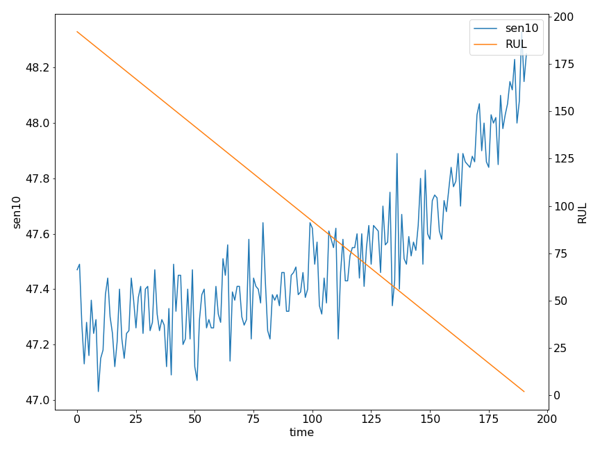
RUL estimation has an additional problem. The data consists of time series of sensor readings from the last repair ($t=0$) to the point of failure ($t_{max}$). The label information here is the remaining lifetime at each step of the time series defined as $RUL(t) = t_{max} - t$. Obviously, we can only calculate the labels if $t_{max}$ is known, i.e. the machine failed. Considering that failure occurs only after significant time, we can see that we accumulate a lot of unlabeled data before we can assign a label.
Abundant unlabeled data cries for semi-supervised learning (SSL) methods, so many approaches were tested in recent years. I found unsupervised pre-training with autoencoders, variational autoencoders, or restricted Boltzmann machines. The basic idea is to take your unlabeled data and use an unsupervised learning technique to get a feature extraction network. Then you add a regression network on top of it and fine-tune the whole thing on your labeled data. The main factor influencing performance here is the amount of available labeled data, so the approaches are tested by using different percentages of the dataset as labeled and the rest as unlabeled. Up until now, reported performance improvements are minimal.
Others took it one step further and used unsupervised domain adaption (UDA) methods. Unsupervised domain adaption can be seen as a generalization of SSL where the labeled and unlabeled data don’t need to be from the same generating distribution. Researchers adopted approaches using adversarial and maximum mean discrepancy metrics that were popularized in the computer vision space. The setup here is to take one subset of your data (divided by working conditions) as labeled and the other as unlabeled. The aim is to minimize the prediction error on the unlabeled data. Performance improvements for these methods are pretty significant, although the performance is still outside the range of where one would consider it for productive use.
Why All of This Doesn’t Matter
Okay, we take established methods from other fields, apply them to ours and get results that are somewhere between negligible and decent. So far, so good. The problem is that none of these results are meaningful at all, because the experimental design was adopted alongside the methods without thinking it through. The offending design choice lies in how the datasets were prepared for these experiments.
There is no RUL estimation benchmark dataset, so researchers made do with adapting existing ones. They took a dataset of labeled time series and partitioned it into a labeled and an unlabeled portion. For the unlabeled portion, they simply discarded the existing labels. If this had been an image dataset, it would be fine, but remember how labels are calculated for RUL estimation. The only thing you need is the time of failure $t_{max}$, and you can label each time step in the series. This means considering any of the time series in our data unlabeled as-is would be highly unrealistic. They can all be labeled trivially. The only reason any time series in our data would be unlabeled is if it did not contain the point of failure. The logical design choice would, therefore, be to discard part of the time series alongside the label, starting at the end of the series.

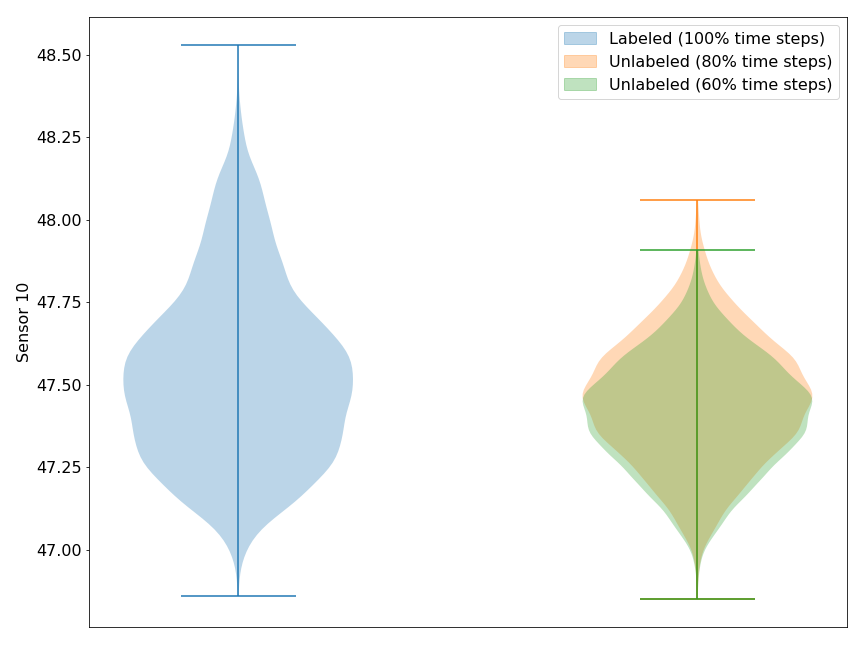
This makes the problem fascinating to work on because it invalidates some assumptions of semi-supervised learning and unsupervised-domain adaption. The figure above shows how the discarded failure data impacts the distribution of an exemplary feature. The distribution shift seems worse going from 100% to 80% than going from 80% to 60%. This trend is consistent when reducing the data even further and underlines the importance of near failure data for capturing the whole feature distribution.
SSL assumes that the labeled and unlabeled data comes from the same generating distribution. Without data from the failure points, the unlabeled data comes from a truncated version of the generating distribution, which may affect training. An autoencoder used for unsupervised pre-training, for example, would focus more on learning the healthy state because it is now even more abundant in the data. This, in turn, leads to worse representations for the failure state.
UDA frees itself from the assumption of matching distributions but still suffers all the same. The UDA methods used up until now are all feature-based, meaning that they try to match the distributions of extracted features from labeled and unlabeled data. The problem here is that we do not only have a distribution shift between labeled and unlabeled data but between training and test data, too, as the test set will contain data near the failure point. In the most extreme case, where we discard a lot of the unlabeled time series, this may lead to a worse performance compared to not using the unlabeled data at all. This is also known as negative transfer.
That UDA methods suffer under these conditions was already shown on the NASA C-MAPSS dataset, a popular RUL estimation benchmark (Link). This is a shameless plug, because it’s, obviously, my own work. We can see in this paper how the performance of the two investigated UDA algorithms degrades with fewer data near failure. If you don’t have access to IEEE Xplore and want a copy of the paper, just shoot me a message.
Lessons Learned
We now see, that the experimental design used for SSL and UDA probably overestimates the test performance, but the fix is relatively simple. Instead of discarding only the label, we discard parts of the unlabeled time series, too. This leads to the question of how much of the time series we can discard or in other words, how far out from failure can a machine be to be useful to our method. The holy grail would be a method that can even draw knowledge from healthy machines alone, but even a method that can use data from machines halfway to failure would be a huge improvement.
On a more general note, we have seen how a whole line of research (albeit a young one) can fall into the trap of blindly copying state-of-the-art methods. As ML practitioners we should definitely draw inspiration and best practices from other fields, but it is no replacement for understanding your data and how your model will be used. There is no need to reinvent the wheel, but you should be certain that a wheel is what you need.
The insights in this post may be mundane and in the end pretty obvious. But you know what they say: in the country of the blindly copying, the one-eyed is king.